ngspice tutorial for beginners

Introduction
Download and Install ngspice (MS Windows)
Download and Install ngspice (Linux)
Circuit with Passive Elements, Operating Point
Circuit with Passive Elements, Transient Simulation
Circuit with Passive Elements, small signal AC Simulation
Download and Install a Simple GUI (MS Windows)
Bipolar Amplifier
Inverting Amplifier with OpAmp
Models and model parameters

ngspice is a circuit simulator that numerically solves equations describing (electronic) circuits: These are made of passive and active devices. Time varying currents and voltages are simulated as well as noise and small signal behavior. ngspice is the Open Source successor of the venerable spice3f5 from UC at Berkeley.

Fig. 1

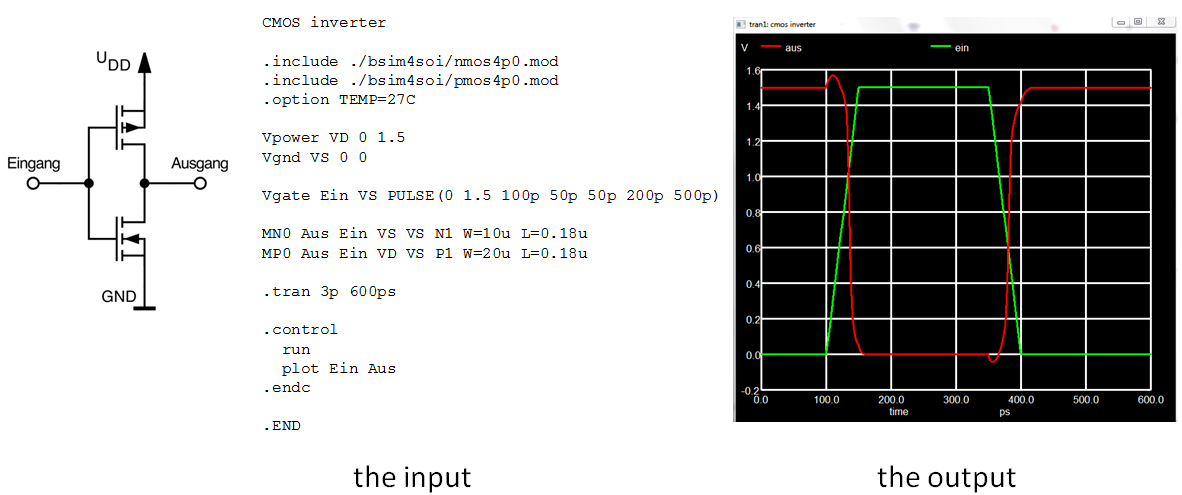
As shown in Fig. 1, you start with a circuit (here: an inverter). You have to create a netlist describing this circuit. The netlist is the input to ngspice, telling it about the circuit to be simulated. Together with some simulation commands this input cares for reading and parsing the netlist, starting the simulation and plotting the output. The output voltage (plotted in red) is the inverse of the (green) input. Both voltages are plotted versus time.

The input to ngspice is read from a file, and it may be enhanced by commands given on the command line. The simulated output may be written to a file, or be plotted as a y-x graph or a smith chart. There is no graphical user interface with schematic capture of circuit diagrams and automatic netlist generation, however there are third party tools available to draw the circuit and generate a ngspice netlist.

There is a detailed reference manual available for ngspice. This manual describes all commands and procedures available in ngspice and lists numerous examples. However, it is not an ngspice how-to or introductory text. This tutorial here gives you some information how to start. If you are interested in getting more in-depth information, you may refer to our book page or to a list of third party tutorials.

Download the zip file for ngspice-43 (about 8.1 MB). Expand this zip file into directory C:\. In MS Windows 10 you might need admin rights to do so. Thus you will get C:\Spice64 with several sub-directories. The main program ngspice.exe resides in folder C:\Spice64\bin.

If you want to make use of PSPICE device models (often provided by the semicondctor companies), put a text file named .spiceinit into your user directory (C:\users\'your name', found also in environmental variable USERPROFILE). Add the two lines


* user provided init file
set ngbehavior=ps

to .spiceinit. If the file name .spiceinit does not work for you, use the alternative file name spice.rc . And that's it!

After a double click on C:\Spice64\bin\ngspice.exe, the ngspice main window pops up.

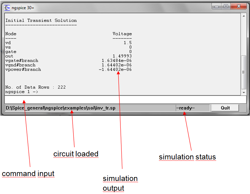
Fig. 2

If you are using LINUX, please check if your distribution already offers a ngspice package for installation. You may then use the distribution's package manager (apt, Yast, etc.) for installation.

If not, you will need to download ngspice-43.tar.gz and compile ngspice with


./configure --with-x --enable-cider --disable-debug CFLAGS="-m64 -O2" LDFLAGS="-m64 -s"
make -j8
sudo make install

or by running the script compile_linux.sh from folder ngspice by


./compile_linux.sh 64

Please check chapt. 28.1 of the ngspice manual for prerequisites and procedures for compiling ngspice-43. After compilation put a text file named .spiceinit into your home/username directory (address to be found also in the environmental variable HOME). In admin mode, it may be the root directory. Add the two lines as noted above to the file.

MacOS users may check for a package available at Homebrew and install ngspice for macOS. MacPorts does offer ngspice as well.

The input and output is now via the console. Below there is a typical view after a transient simulation of a circuit.


******
** ngspice-35 : Circuit level simulation program
** The U. C. Berkeley CAD Group
** Copyright 1985-1994, Regents of the University of California.
** Copyright 2001-2020, The ngspice team.
** Please get your ngspice manual from https://ngspice.sourceforge.io/docs.html
** Please file your bug-reports at https://ngspice.sourceforge.io/bugrep.html
** Creation Date: Aug  8 2021   22:01:36
******
ngspice 6 -> source /home/holger/software/ngspice/examples/soi/inv_tr.sp

Circuit: soi inverter

Doing analysis at TEMP = 27.000000 and TNOM = 27.000000


Initial Transient Solution
--------------------------

Node                                   Voltage
----                                   -------
vd                                         1.5
vs                                           0
gate                                         0
out                                    1.49993
vgate#branch                       1.63484e-06
vgnd#branch                        1.64402e-06
vpower#branch                     -1.64402e-06

No. of Data Rows : 222
ngspice 7 ->

Now let's do a first circuit. We need a dc voltage source and two resistors that build a simple resistive voltage divider.

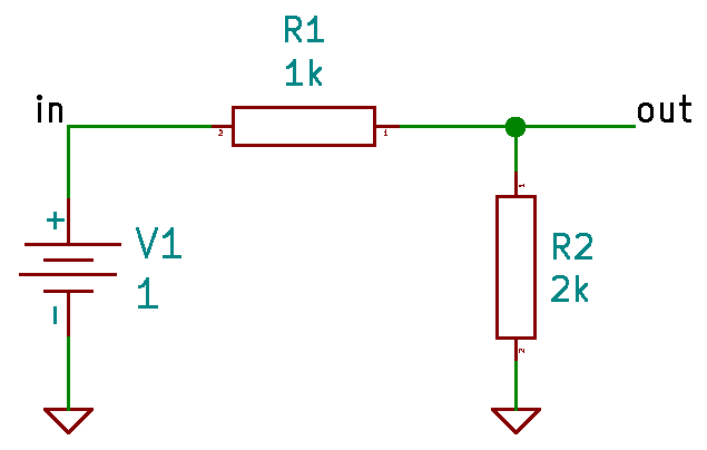
Fig. 3

What is the netlist of this circuit? The voltage source is connected between 0 (ground) and node 'in', value 1, R1 between 'in' and 'out' with value 1k, R2 between 'out' and ground and value 2k.


voltage divider netlist
V1 in 0 1
R1 in out 1k
R2 out 0 2k
.end

Line 1 is a title line. .end in line 5 denotes the end of the netlist. Put these lines into a text file named vdiv.cir and save it to the folder C:\Spice64\bin (If you are with MS Windows). Now start ngspice by double click onto ngspice.exe in C:\Spice64\bin. Load the netlist into ngspice by entering the command source vdiv.cir. ngspice is now ready for simulation, the netlist is loaded. What kind of simulation do we now want to have? Of interest is the DC voltage at node "out". This is the operating point of the circuit. We will get this by entering the op command. Then we want to get the voltage value at node "out". Let's enter the print out command. This is the output you will get with ngspice for the complete sequence, and you see the voltage at node "out":


******
** ngspice-31 : Circuit level simulation program
** The U. C. Berkeley CAD Group
** Copyright 1985-1994, Regents of the University of California.
** Please get your ngspice manual from https://ngspice.sourceforge.io/docs.html
** Please file your bug-reports at https://ngspice.sourceforge.io/bugrep.html
** Creation Date: Mar 30 2019   09:37:02
******
ngspice 1 -> source vdiv.cir

Circuit: voltage divider netlist

ngspice 2 -> op
Doing analysis at TEMP = 27.000000 and TNOM = 27.000000

No. of Data Rows : 1
ngspice 3 -> print out
out = 6.666667e-01
ngspice 4 ->

If you are with Linux, you might put vdiv.cir into a folder of your choice. Then cd into that folder and call ngspice from your command line window. You will not need the source command, when you directly call


ngspice vdiv.cir

Then the circuit is loaded immediately, and the next command you enter is op (see above).

The following example is a dual rc ladder, and we want to do a transient simulation. The input is a voltage waveform (a pulse) versus time, and the output is a waveform as well, as you might see on an oscilloscope. This is our circuit:

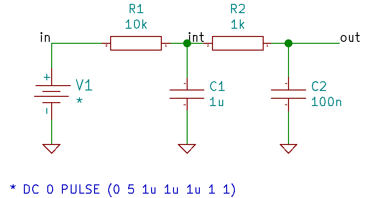
Fig. 4

The netlist then is


.title dual rc ladder
R1 int in 10k
V1 in 0 dc 0 PULSE (0 5 1u 1u 1u 1 1)
R2 out int 1k
C1 int 0 1u
C2 out 0 100n
.end

We have to talk about the voltage source V1. In the previous example it just emits a constant 1V. Now it is more complex. The manual says in chapt. 4.1.1: For a pulse we have to add PULSE(VL VH TD TR TF PW PER PHASE) to the DC voltage of our voltage source, where VL is the starting, VH the end voltage, TD a delay, TR and TF are rise and fall times, PW is the pulse width, PER the period of repetition, PHASE a phase shift. We have a pulse from 0 to 5 V, the delay before the pulse starts, its rise and fall times are all 1 us. Pulse width and pulse period are 1 s each, far beyond our intended simulation time. Phase does not matter here, we omit it. So here we apply just the rising edge of the pulse.

What is now the simulation time we will need? The time constant of our low pass filter is dominated by R1C1 and is about 1uF*10kOhm = 10ms. So we might be well off by starting at 0 and simulate until 50 ms. We should use 1000 points, so step size is 50 us. Thus, when you have loaded the circuit, the simulation command now is


tran 50u 50m

The result is shown in Fig. 5 after plotting with command plot in int out. The voltages at nodes 'int' and 'out' barely differ. This is because the first R1C1 dominates the circuit. The time constant of the second R2C2 is a factor of 100 smaller, so charging C2 is quick and easy compared to charging C1. The voltage at input node 'in' rises so fast that you do not see its slope.

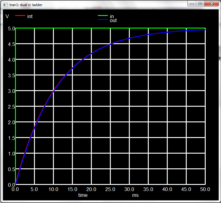
Fig. 5

Now we want to see what the small signal behavior of this rc ladder network might be. Small signal means that we set a dc operating point to our circuit. Then we add a small ac signal to the input and simulate what the output ac voltage might be versus frequency. So we have to vary the frequency of this small input signal. And we are not interested at the absolute output voltage value, but its relation to the input (gain) and its phase shift in relation to the input (phase). Fortunately there is the 'ac' command in ngspice that makes life easy. Firstly we have to tell ngspice where to input their small signal ac voltage. We choose node 'in', that is our voltage source V1. V1 now becomes


V1 in 0 dc 0 ac 1 PULSE (0 5 1u 1u 1u 1 1)

We simply added 'ac 1'. The 'dc 0' sets the operating point (which does not matter because of our simple circuit), 'PULSE' does matter only during transient simulation, so we keep it for simplicity. The 1 in 'ac 1' just helps us getting the ratio out/in, by dividing the output by 1, or just take it as is. The simulation command is


ac dec 10 1 100k

We want to do an 'ac' simulation. We vary the frequency as if plotted logarithmically, with 10 points per decade. The starting frequency is 1 Hz, the stopping frequency is 100 kHz. So we will get 51 data points. If now plotted with the command plot out, the graph looks ugly (output below 0?). Well, we are dealing with ac signals. These are complex numbers, consisting of a real part and an imaginary part (or equivalently consist of magnitude and phase). Traditionally plot out only delivers the real part of the signal. But we want to see magnitude (or gain) and phase, like in a Bode plot. So one should use plot vdb(out) for the gain in dB and plot ph(out) for the phase. Now the graphs are o.k., but titles and labels are not yet satisfactory. ngspice plotting procedures here need some manual tweaking.

But before we move on, we have to streamline our approach. Typing everything to the console seems to be annoying. ngspice has a mechanism to assemble all interactive commands (the ones we have typed) into a .control ... .endc section. This .control section may be added to the netlist, which now looks like


.title dual rc ladder
* file name rcrcac.cir
R1 int in 10k
V1 in 0 dc 0 ac 1 PULSE (0 5 1u 1u 1u 1 1)
R2 out int 1k
C1 int 0 1u
C2 out 0 100n

.control
ac dec 10 1 100k
plot vdb(out)
plot ph(out)
.endc

.end

We now may start ngspice by ngspice rcrcac.cir. The netlist is read, the commands in the .control section (ac simulation and plotting) are executed automatically. Still we would like to improve the graphics plot. We do this by using several extra commands, that we add to the .control section. All of them are described in the ngspice manual, chapt. 13.5. The complete input file now reads:


.title dual rc ladder
* file name rcrcac.cir
R1 int in 10k
V1 in 0 dc 0 ac 1 PULSE (0 5 1u 1u 1u 1 1)
R2 out int 1k
C1 int 0 1u
C2 out 0 100n

.control
ac dec 10 1 100k
settype decibel out
plot vdb(out) xlimit 1 100k ylabel 'small signal gain'
settype phase out
plot cph(out) xlimit 1 100k ylabel 'phase (in rad)'
let outd = 180/PI*cph(out)
settype phase outd
plot outd xlimit 1 100k ylabel 'phase'
.endc

.end

And this is what we see after simulation and plotting:

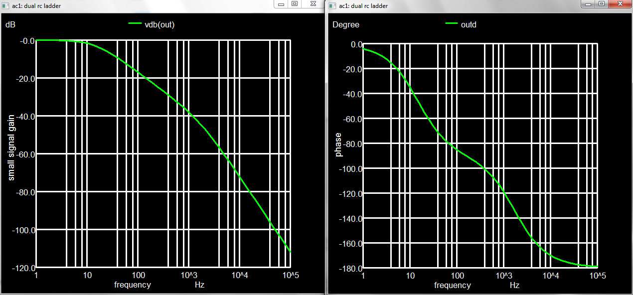
Fig. 6 Small Signal Magnitude and Phase for dual RC ladder

I am used to MS Windows, and so I do not want to type in everything, but use the mouse to select files, start simulation and plot the results. Therefore I use (and have made available for download) a small GUI that is shown in Fig. 7. To install, just expand the four files into a folder of your choice. DuSpiceStart.exe is the main executable. DuSpicePlot.exe reads a raw file and prepares plotting. DuSpiceStart.ini contain the setup data. plot_spex3.xlsm contains some VB macros that allow plotting with EXCEL.

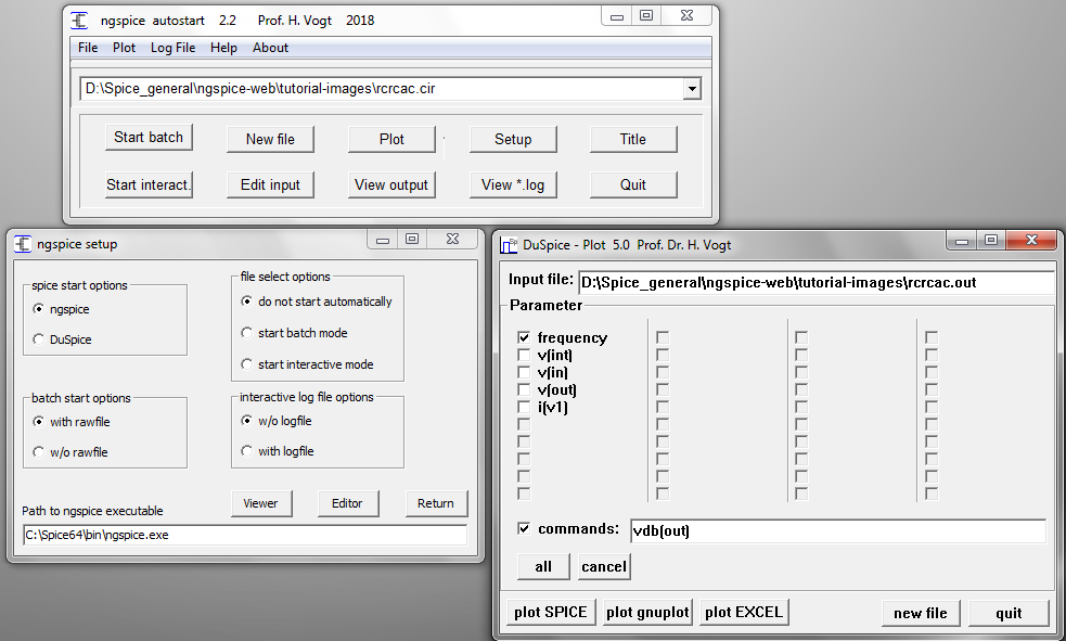
Fig. 7 MS Windows GUI with Setup and Plot Window

If you hover your mouse over a button or edit box, a small hint will pop up and give you some information on the usage of this item.

Main window: Drop down box on top: Select one of the recent 5 files as input for simulation

Start batch: Start ngspice in batch mode, like ngspice -b -r rcrcac.out -o rcrcac.log rcrcac.cir

New file: Select a new input file (e.g. rcrcac.cir)

Plot: Open the Plot window by calling DuSpicePlot.exe, only useful if simulation has been run before in batch mode

Setup: Open the Setup window

Title: Show the title line of the input file

Start interact.: Start ngspice in interactive mode

Edit input: Open the input file in the editor

View output: Open the output file (e.g. rcrcac.out) in the editor

View *.log: Open the log file (e.g. rcrcac.log) in the editor

Quit: Quit the GUI

Setup window: Viewer: Select a file viewer (recommended: Notepad++)

Editor: Select an editor (recommended: Notepad++)

Return: Back to Main window

Path to ngspice executable: Double click on edit box to select ngspice path and executable

Spice start options: Select ngspice or another spice

file select options: Start ngspice automatically in interactive or in batch mode, or do not start automatically and wait for user to start ngspice from main window

batch start options: If 'Start batch' from main window is selected, start either with rawfile (e.g. -r rcrcac.out) or without. Then output gets into rcrcac.log only (like the ancient printer plot)

interactive log file options: Start interactive simulation either with output going to the ngspice output window or into the log file

Plot window: plot Spice: Start another instance of ngspice, load the *.out file and start plotting

plot gnuplot: Start gnuplot (if available) and start plotting

plot EXCEL: Start MS EXCEL (if available) and start plotting

all: select all output vectors for plotting

cancel: unselect all output vectors

commands: Check the check box and type in any vector or allowed function of a vector to be plotted. All parameters that are valid following the 'plot' command are allowed.

input file: Show the output (raw) file selected for plotting

new file: Select a new raw file for plotting

quit: Quit plot window

The next example is a bipolar amplifier. A npn bipolar transistor BC546 is the amplifying device. Two resistors R1, R2 determine the base current, R3 is the dc load resistor. RLoad is required because ngspice will not accept a capacitor that does not have a dc connection at each terminal. VCC is the power supply, Vin the input voltage source.

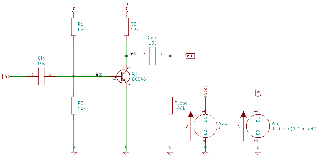
Fig. 8

Even with all devices assembled as shown, the circuit is not complete. The transistor Q1 will need more data for simulation. The bipolar transistor model (equations to calculate currents as function of terminal voltages) is hard-coded in ngspice. This model however requires model parameters to make these calculations specific for the transistor that was selected (BC546). These data are not delivered with ngspice. They are device manufacturer specific and may be obtained from their web sites or from other sites (here e.g. from BC546 model parameters, see also the spice model collection from our model parameters page for many more). What do we get from there?


.model BC546B npn ( IS=7.59E-15 VAF=73.4 BF=480 IKF=0.0962 NE=1.2665
+ ISE=3.278E-15 IKR=0.03 ISC=2.00E-13 NC=1.2 NR=1 BR=5 RC=0.25 CJC=6.33E-12
+ FC=0.5 MJC=0.33 VJC=0.65 CJE=1.25E-11 MJE=0.55 VJE=0.65 TF=4.26E-10
+ ITF=0.6 VTF=3 XTF=20 RB=100 IRB=0.0001 RBM=10 RE=0.5 TR=1.50E-07)

It is a line starting with .model, followed by its corresponding name BC546B and the device type, that is a npn transistor. In brackets then we have all the model parameters that, in coalition with the hard coded model, will yield the dc, ac, transient or noise behavior of the transistor. All of the line might come in a single row. For readability reasons you might want to split this overly long line into e.g. four. Each consecutive line the has to start with a +. Internally ngspice adds all of the consecutive lines into a single one. The resulting netlist (file bipamp.cir) is


bipolar amplifier
* file bipamp.cir
.model BC546B npn ( IS=7.59E-15 VAF=73.4 BF=480 IKF=0.0962 NE=1.2665
+ ISE=3.278E-15 IKR=0.03 ISC=2.00E-13 NC=1.2 NR=1 BR=5 RC=0.25 CJC=6.33E-12
+ FC=0.5 MJC=0.33 VJC=0.65 CJE=1.25E-11 MJE=0.55 VJE=0.65 TF=4.26E-10
+ ITF=0.6 VTF=3 XTF=20 RB=100 IRB=0.0001 RBM=10 RE=0.5 TR=1.50E-07)
R3 vcc intc 10k
R1 vcc intb 68k
R2 intb 0 10k
Cout out intc 10u
Cin intb in 10u
VCC vcc 0 5
Vin in 0 dc 0 ac 1 sin(0 1m 500)
RLoad out 0 100k
Q1 intc intb 0 BC546B
.tran 10u 10m
*.ac dec 10 10 1Meg
.end

The .model line directly corresponds with the Q1 line in that it now delivers the necessary model parameters. With the line .tran 10u 10m the netlist contains another new element, again a dot command. This is useful if you want to run ngspice in batch mode. The next line *.ac dec 10 10 1Meg is prepended by *. This serves for commenting out the line. Each line starting with * is treated as a comment and is ignored during simulation. Placing the * allows selecting a simulation type.

If you are on MS Windows, start the GUI, New file bipamp.cir, Start batch, Plot, check v(out) and v(in), plot gnuplot: this is the result:

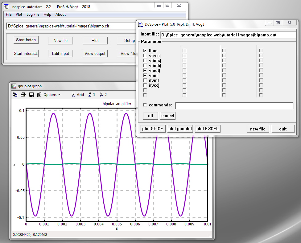
Fig. 9 GUI, Plot window and gnuplot graph

With Linux you might add a .control section like


.control
run
gnuplot gp v(out) v(in)
.endc

to the input file bipamp.cir. Then cd into the folder containing the input file and start the simulation by ngspice bipamp.cir.

The final example is an inverting amplifier using the operational amplifier LF356. Its gain is set by the ratio of R2 to R1. The amplifier inverts the input polarity. Thus the output will be V(out) = -R2/R1*V(in) = -100*V(in).

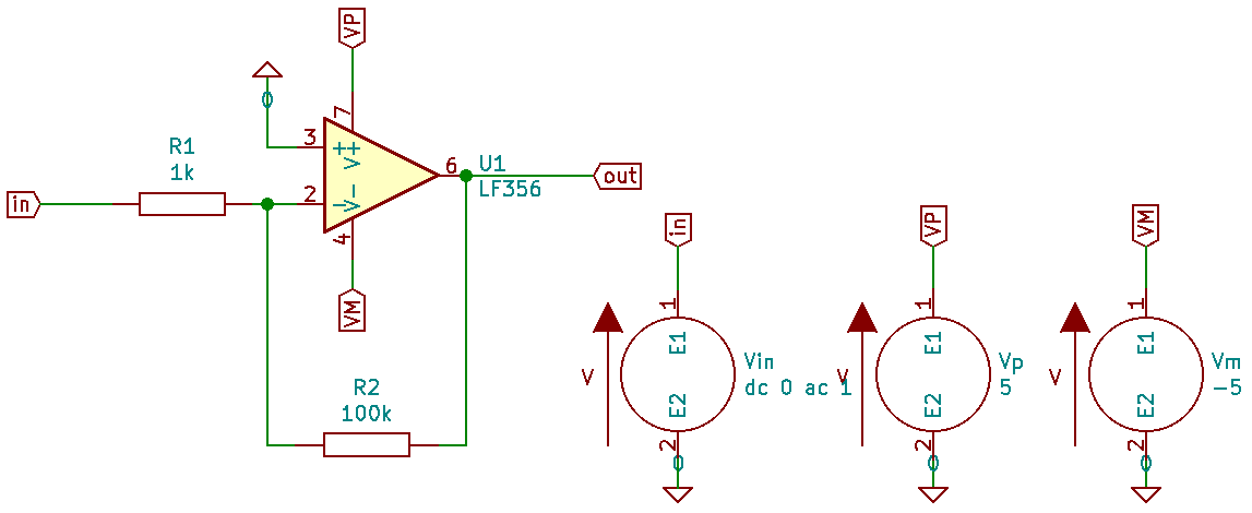
Fig. 10 Inverting amplifier with OpAmp

There is no model for OpAmps delivered with ngspice. So you have to search in the web for a device manufacturer's model, e.g. from the TI web pages as LF356.mod. A wealth of models for discretes and ICs from the early 2000s is available at the ngspice model collection and its sub-folders.

If you have a look at LF356.mod, there you find the circuit assembled in a subcircuit (between the .subckt and the .ends lines) with name LF356/NS and 5 connecting nodes.

How to add the LF356 model to the ngspice netlist? Copy the file LF356.mod into the folder that will also contain the netlist OpAmp.cir. Add the line .include LF356.mod to the netlist file OpAmp.cir.

How to invoke the model in the netlist? This is done by an X line (see manual chapt. 2.4) like XU1 3 2 7 4 6 LF356/NS. The pin numbers correspond to the pins of the IC as found in its data sheet. We have decided to use the pin numbers as node names for the netlist. We might have chosen other net names (e.g. the circuit pin names) as well. The 'circuit pin name'/'pin number' pairs are in- / 2, in+ / 3, V+ / 7, V- / 4, and out / 6. The model requires a sequence

non-inverting input
inverting input
positive power supply
negative power supply
output

as described in the model file. Therefore the nodes in the X line have to be ordered into this sequence, i.e. 3 2 7 4 6. The complete netlist now looks like:


.title Inverting OpAmp amplifier
*file OpAmp.cir
.include LF356.MOD
XU1 3 2 7 4 6 LF356/NS
R1 2 in 1k
Vin in 0 dc 0 ac 1
Vp 7 0 5
Vm 4 0 -5
Vin+ 3 0 0
R2 6 2 100k
.end

This time we want to do a dc simulation, that is we vary the input with a slightly rising dc voltage and measure the output. One has to remember that the power supply delivers +-5 V, so the output can't be larger, and the amplification is -100. So we use the command dc Vin -50m 50m 2m to vary Vin from -50 mV to 50 mV with a step size of 2 mV. We may either add the command


.dc Vin -50m 50m 2m

to our netlist and use the GUI, or we add the .control section


.control
dc Vin -50m 50m 2m
plot v(in) v(6)
.endc

to the netlist, cd into this input folder and run


ngspice OpAmp.cir

in the Cygwin or Linux console. The plotted output then is

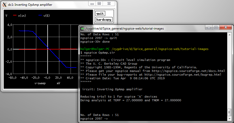
Fig. 11 OpAmp dc simulation in and out

The input voltage variation is barely to be seen. The OpAmp output saturates already at +-3 V, far away from rail-to-rail +-5 V which is possible with modern OpAmps.

A final remark: If you want a GUI with schematic capture (that is entering the input via a circuit diagram, not by the netlist), we recommend KiCAD. An introductory tutorial for ngspice in KiCAD is Ngspice using KiCad/Eeschema GUI for schematic entry, simulation and plotting.

For a ngspice simulation ngspice expects as input a netlist, simulation parameters, an output selection, and simulation models or parameters for the devices used in the netlist. A comprehensive selection of models and model parameters is found on our ngspice model and model parameter page. Especially the two collections

will give you almost everything needed.