Ngspice circuit simulator - TCLspice learning by examples

TCLspice comes as a library for TCL langugage. This is not (really) a TCL lesson, neither a TCLspice lesson. If you have not done it before, read TCLspice user manual. It is both short and comprehensive. It contains a bibliography of interest.

This document will present you some useful applications to kickstart you. The tarball of the examples can be downloaded here. Three example are provided:

Active capacitor measurement
Optimisation of a linearization circuit for a Thermistor
Progressive display

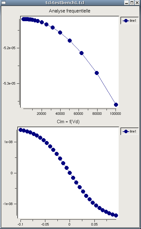
In this crude implementation of a circuit described by Marc KODRNJA. This simulation outputs a graph representing the virtual capacitance versus the command voltage. The function C=f(V) is calculated point by point. For each control voltage value, the virtual capacitance is calculated with the voltage and intensity accross the output port in a frequency simulation. A control value that should be as close to zero as possible is calculated to assess simulation success.

This script can be invoked by typing wish testbench1.tcl

testbench1.tcl

This line loads the simulator capabilities

package require spice

This is a comment (Quite useful if you intend to live with other Human beings)

# Test of virtual capacitore circuit # Vary the control voltage and log the resulting capacitance

A good example of the calling of a spice command: preceed it with spice::

spice::source "testCapa.cir"

This reminds that any regular TCL command is of course possible

set n 30 set dv 0.2 set vmax [expr $dv/2] set vmin [expr -1 * $dv/2] set pas [expr $dv/ $n]

BLT vector is the structure used to manipulate data. Instantiate the vectors

blt::vector create Ctmp blt::vector create Cim blt::vector create check blt::vector create Vcmd

Data is in my coding style plotted into graph objects. Instantiate the graph

blt::graph .cimvd -title "Cim = f(Vd)" blt::graph .checkvd -title "Rim = f(Vd)" blt::vector create Iex blt::vector create freq blt::graph .freqanal -title "Analyse frequentielle" # # First simulation: A simple AC plot # set v [expr {$vmin + $n * $pas / 4}] spice::alter vd = $v spice::op spice::ac dec 10 100 100k

Retrieve a the intensity of the current accross Vex source

spice::vectoblt {Vex#branch} Iex

Retrieve the frequency at wich the current have been assessed

spice::vectoblt {frequency} freq

Room the graph in the display window

pack .freqanal

Plot the function Iex =f(V)

.freqanal element create line1 -xdata freq -ydata Iex # # Second simulation: Capacitance versus voltage control # for {set i 0} {[expr $n - $i]} {incr i } { set v [expr {$vmin + $i * $pas}] spice::alter vd = $v spice::op spice::ac dec 10 100 100k

Image capacitance is calculated by spice, instead of TCL there is no objective reason

spice::let Cim = real(mean(Vex#branch/(2*Pi*i*frequency*(V(5)-V(6))))) spice::vectoblt Cim Ctmp

Build function vector point by point

Cim append $Ctmp(0:end)

Build a control vector to check simulation success

spice::let err = real(mean(sqrt((Vex#branch-(2*Pi*i*frequency*Cim*V(5)-V(6)))^2))) spice::vectoblt err Ctmp check append $Ctmp(0:end)

Build abscissa vector

Vcmd append $v }

Plot

pack .cimvd .cimvd element create line1 -xdata Vcmd -ydata Cim pack .checkvd .checkvd element create line1 -xdata Vcmd -ydata check

This example is both the first and the last optimization program I wrote for an electronic circuit. It is far from perfect.

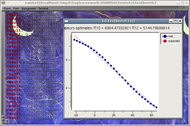
The temperature response of a CTN is exponential. It is thus nonlinear. In a battery charger application floating voltage varies linearly with temperature. A TL431 voltage reference sees its output voltage controlled by two resistors (r10, r12) and a thermistor (r11). The thermistor is modeled in spice by a regular resistor. Its resistivity is assessed by the TCL script. It is set with a spice::alter command. This script uses an iterative optimization approach to try to converge to a set of two resistor values which minimizes the error between the expected floating voltage and the TL431 output.

This script can be executed by the user by simply executing the file in a terminal.

./testbench3.tcl

Two issues are important to point out: Graphical display of the current temperature response is not yet possible and I don't know why. Each time a simulation is performed, some memory is allocated for it. The simulation result remains in memory until the libspice library is unloaded (typically the tcl script ends) or when a spice::clean command is performed. In this kind of simulation, not cleaning the memory space will freeze your computer and you'll have to restart it.

For those who are really interesting in optimizing circuits: Some parameters are very important for quick and correct convergence: The optimizer walks step by step to a local minimum of the cost function you define. Starting from an initial vector YOU provide it, it converges step by step. Consider trying another start vector if the result is not the one you expected. The optimizer will carry on walking until it reaches a vector which resulting cost is smaller than the target cost YOU provide it. You will also provide a maximum iteration count in case the target can not be achieved. Balance your time, specifications, and every other parameters to set both. For a balance between quick and accurate convergence adjust the "factor" variable, at the beginning of minimumSteepestDescent in the file differentiate.tcl.

This calls the shell sh who then runs wish with the file itself.

#!/bin/sh # WishFix \ exec wish "$0" ${1+"$@"} ###

Regular package for simulation

package require spice

Here the important line is source differentiate.tcl which contains optimisation library

source differentiate.tcl

Generates a temperature vector

proc temperatures_calc {temp_inf temp_sup points} { set tstep [ expr " ( $temp_sup - $temp_inf ) / $points " ] set t $temp_inf set temperatures "" for { set i 0 } { $i < $points } { incr i } { set t [ expr { $t + $tstep } ] set temperatures "$temperatures $t" } return $temperatures }

generates thermistor resistivity as a vector, typically run: thermistance_calc res B [ temperatures_calc temp_inf temp_sup points ]

proc thermistance_calc { res B points } { set tzero 273.15 set tref 25 set thermistance "" foreach t $points { set res_temp [expr " $res * exp ( $B * ( 1 / ($tzero + $t) - 1 / ( $tzero + $tref ) ) ) " ] set thermistance "$thermistance $res_temp" } return $thermistance }

generates the expected floating value as a vector, typically run: tref_calc res B [ temperatures_calc temp_inf temp_sup points ]

proc tref_calc { points } { set tref "" foreach t $points { set tref " $tref [ expr " 6 * (2.275-0.005*($t - 20) ) - 9" ] " } return $tref }

In the optimisation algorithm, this function computes the effective floating voltage at the given temperature.

### NOTE: ### As component values are modified by a spice::alter Component values can be considered as global variable. ### R10 and R12 are not passed to iteration function because it is expected to be correct, ie to have been modified soon before proc iteration { t } { set tzero 273.15 spice::alter r11 = [ thermistance_calc 10000 3900 $t ] #spice::set temp = [ expr " $tzero + $t " ] spice::op spice::vectoblt vref_temp tref_tmp ###NOTE: ###As the library is executed once for the whole script execution, it is important to manage the memory ###and regularly destroy unused data set. The data computed here will not be reused. Clean it spice::destroy all return [ tref_tmp range 0 0 ] }

This is the cost function optimization algorithm will try to minimize. It is a square norm of the error accross the temperature range [-25:75]°C (square norm: norme 2 in french I'm not sure of the english translation)

proc cost { r10 r12 } { tref_blt length 0 spice::alter r10 = $r10 spice::alter r12 = $r12 foreach point [ temperatures_blt range 0 [ expr " [temperatures_blt length ] - 1" ] ] { tref_blt append [ iteration $point ] } set result [ blt::vector expr " 1000 * sum(( tref_blt - expected_blt )^2 )" ] disp_curve $r10 $r12 return $result }

This function displays the expected and effective value of the voltage, as well as the r10 and r12 resistor values

proc disp_curve { r10 r12 } { .g configure -title "Valeurs optimales: R10 = $r10 R12 = $r12" }

Main loop starts here

# # Optimization # blt::vector create tref_tmp blt::vector create tref_blt blt::vector create expected_blt blt::vector create temperatures_blt temperatures_blt append [ temperatures_calc -25 75 30 ] expected_blt append [ tref_calc [temperatures_blt range 0 [ expr " [ temperatures_blt length ] - 1" ] ] ] blt::graph .g pack .g -side top -fill both -expand true .g element create real -pixels 4 -xdata temperatures_blt -ydata tref_blt .g element create expected -fill red -pixels 0 -dashes dot -xdata temperatures_blt -ydata expected_blt

Source the circuit and optimize it, result is retrieved in r10r12 variable and affected to r10 and r12 with a regular expression. A bit ugly.

spice::source FB14.cir set r10r12 [ ::math::optimize::minimumSteepestDescent cost { 10000 10000 } 0.1 50 ] regexp {([0-9.]*) ([0-9.]*)} $r10r12 r10r12 r10 r12

Outputs optimization result

# # Results # spice::alter r10 = $r10 spice::alter r12 = $r12 foreach point [ temperatures_blt range 0 [ expr " [temperatures_blt length ] - 1" ] ] { tref_blt append [ iteration $point ] } disp_curve $r10 $r12

This example is quite simple but it is very interesting. It displays a transient simulation result on the fly. You may now be familiar with most of the lines of this script. It uses the ability of BLT objects to automatically update. When the vector data is modified, the stripchart display is modified accordingly.

#!/bin/sh # WishFix \ exec wish -f "$0" ${1+"$@"} ### package require BLT package require spice

this avoids to type blt:: before the blt class commands

namespace import blt::* wm title . "Vector Test script" wm geometry . 800x600+40+40 pack propagate . false

A strip chart with labels but without data is created and displayed (packed)

stripchart .chart pack .chart -side top -fill both -expand true .chart axis configure x -title "Time" spice::source example.cir spice::bg run after 1000 vector create a0 vector create b0 vector create a1 vector create b1 vector create stime proc bltupdate {} { puts [spice::spice_data] spice::spicetoblt a0 a0 spice::spicetoblt b0 b0 spice::spicetoblt a1 a1 spice::spicetoblt b1 b1 spice::spicetoblt time stime after 100 bltupdate } bltupdate .chart element create a0 -color red -xdata stime -ydata a0 .chart element create b0 -color blue -xdata stime -ydata b0 .chart element create a1 -color yellow -xdata stime -ydata a1 .chart element create b1 -color black -xdata stime -ydata b1