


Tutorial: ngspice control language
- Introduction
- Inverter as example circuit
- Multiple simulations in a single run
- Looping a simulation, altering the supply voltage
- About plots, variables and vectors
- Looping a simulation, plot the maximum gain versus supply voltage
- Looping the simulation as in 5., no plot, write data to file only
- About loops in general
- String substitution
- Nested loops
- Emulate nested .step commands
- Modify a circuit on the fly
- More examples
0. Introduction
ngspice circuit simulator offers a built-in control language (formerly know as nutmeg language). It allows to create scripts which automate the simulation flow and provide support for simulation data analysis.
There are three basic methods to start a simulation with ngspice. The traditional method is
the batch mode. With an input netlist given (see below), the command
ngspice -b -r inv-example.raw inv-example.cir will start the simulation, executing the dot commands from the netlist,
saving the simulation data in the 'raw' file, without any further user interaction. On the other hand we have
the interactive mode. You start ngspice by ngspice inv-example.cir. ngspice sources the netlist and then waits
for user input. You may type any of the commands found in chapter 13.5 of the
ngspice manual or the ngspice xhtml manual
to initiate some action (e.g. running the simulation, plotting or saving the data etc.). The real power
of using these commands however is unfolded in the third mode of running ngspice, the control mode.
You assemble a sequence of commands into a script, add this script to the netlist, and then start ngspice as usual by
ngspice inv-example.cir. ngspice will execute the commands from the script, enabling multiple
simulations, loops, data processing, plotting and saving data. About 100 commands are available, scripts may range
from simple ones with few lines up to complex ones with several hundred commands.
And this is what the tutorial is about: How to use the control language for efficient simulations by unfolding the power of ngspice.
Several examples will be given, beginning with simple support scripts to run a simulation and plot the results, up to some more advanced techniques. You may copy the examples (netlist and control sections) and paste them into your input files to run simulation "experiments".
The tutorial is not yet complete, is a work-in-progress, and user input is welcome to enhance it further. Please use the discussion forum for feedback and questions.
More info on starting ngspice is available in chapter 12.4 of the ngspice manual. ngspice download and installation is described in the ngspice tutorial. Commands used in the scripts below are not all explained in detail, please use the ngspice manual chapter 13.5 as your reference.
1. Inverter as an example circuit
Throughout the tutorial we will use a very simple circuit, a CMOS inverter with 2 transistors (NMOS and PMOS). The netlist is (comment lines are starting with *, end-of-line comments with ;):
inverter example circuit for control language tutorial
* file inv-example.cir

* the power supply 2.0 V
Vcc cc 0 2

* the input signal for dc and tran simulation
Vin in 0 dc 0 pulse (0 2 95n 2n 2n 90n 180n)

* the circuit
Mn1 out in 0 0 nm W=2u L=0.18u
Mp1 out in cc cc pm W=4u L=0.18u

* model and model parameters (we use the built-in default parameters for BSIM4)
.model nm nmos level=14 version=4.8.1
.model pm pmos level=14 version=4.8.1

* simulation commands
.tran 100p 500n

* control language script
.control                                    ; begin of control section
run                                         ; run the .tran command
set xbrushwidth=2                           ; set linewidth of graph
plot v(in) v(out)                           ; plot the simulation results
write $inputdir/simout.out v(in) v(out)     ; write the results to a file
.endc                                       ; end of control section

.end
The dot command .tran 100p 500n sets the simulation type (transient) and its parameter range
(time 0 to 500 ns, step 100 ps). There is already a control script added to the netlist file: enclosed in
.control ... .endc there are commands like run to execute the simulation,
set xbrushwidth=2 to increase the linewidth of the graph plotted, and write $inputdir/simout.out
v(out) to write the output voltage into a file located in the input directory, where input file inv-example.cir
stems from.
2. Multiple simulations in a single run
If you want to execute more than one simulation in a single run, it might be advisable not to use
the dot command .tran 100p 500n, but its equivalent control command tran 100p 500n
(no dot!) inside of the control section (replacing run):
inverter example circuit for control language tutorial
* file inv-example2.cir

* the power supply 2.0 V
Vcc cc 0 2

* the input signal for dc and tran simulation
Vin in 0 dc 0 pulse (0 2 95n 2n 2n 90n 180n)

* the circuit
Mn1 out in 0 0 nm W=2u L=0.18u
Mp1 out in cc cc pm W=4u L=0.18u

* model and model parameters (we use the built-in default parameters for BSIM4)
.model nm nmos level=14 version=4.8.1
.model pm pmos level=14 version=4.8.1

* control language script
.control
tran 100p 500n               ; simulation command 1
set xbrushwidth=2
plot v(in) v(out)
write $inputdir/outtran.out v(in) v(out)
reset
dc vin 0 2 0.01              ; simulation command 2
plot v(out)                  ; v(in) not required because it is the x axis already
write $inputdir/outdc.out v(out)
.endc
.end
Fig. 1 is what you get with the two plot commands:
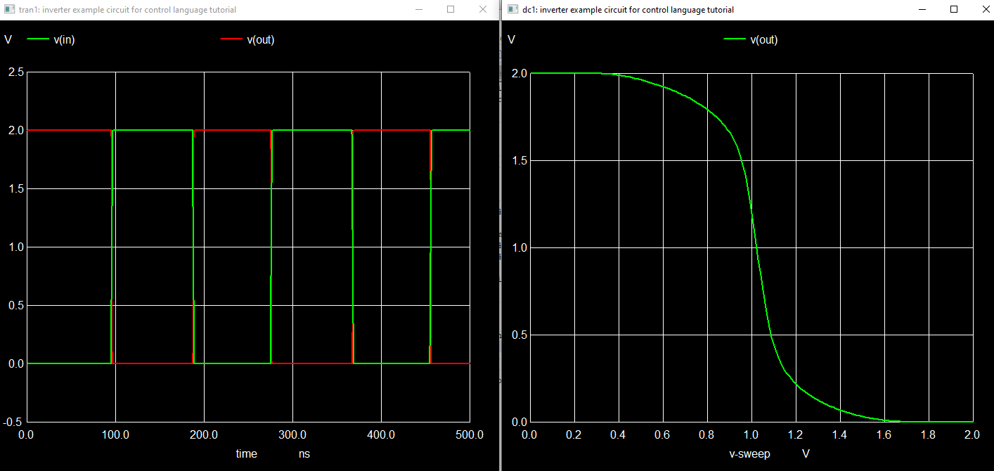
Fig. 1 Inverter input/output versus time and inverter output versus input voltage
Command reset is required to set back internal data after a transient simulation. If you do not want a graphical output, but just the output into a file, you might modify the script by adding the quit command:
* control language script
.control
tran 100p 500n               ; simulation command 1
write $inputdir/outtran.out v(in) v(out)
reset
dc vin 0 2 0.01              ; simulation command 2
write $inputdir/outdc.out v(out)
quit
.endc
.end
Now after finishing the control script, ngspice exits immediately. Therefore plotting
does not make sense (except for using the gnuplot command, when gnuplot is installed).
3. Looping a simulation, altering the supply voltage
The next script executes a repeat loop. For five times the inverter supply voltage is changed, each time a new dc simulation is run. Finally all dc simulation results are plotted in a single plot. In addition we plot the inverter gain and its current consumption during the dc sweep.
* control language script
.control
let vccc = 1.2            ; create a vector vccc and assign value 1.2
repeat 5                  ; loop start
  alter Vcc $&vccc        ; alter the voltage Vcc using vector vccc
  dc vin 0 2 0.01         ; run the dc simulation
  let vccc = vccc + 0.2   ; calculate new voltage value for Vcc by updating vector vccc
end                       ; loop end, jump back to loop start
set xbrushwidth=2         ; assign value 2 to the predefined variable
plot dc1.v(out) dc2.v(out) dc3.v(out) dc4.v(out) dc5.v(out)
set nounits               ; do not plot units on the x and y axes.
plot deriv(dc1.v(out)) deriv(dc2.v(out)) deriv(dc3.v(out)) deriv(dc4.v(out)) deriv(dc5.v(out)) ylabel 'Inverter gain V / V' xlabel 'vsweep V'
unset nounits             ; undo the previous set command
plot dc1.I(vcc) dc2.I(vcc) dc3.I(vcc) dc4.I(vcc) dc5.I(vcc) ylabel 'Inverter current consumption'
.endc
Fig. 2 is the result of the three plot commands:
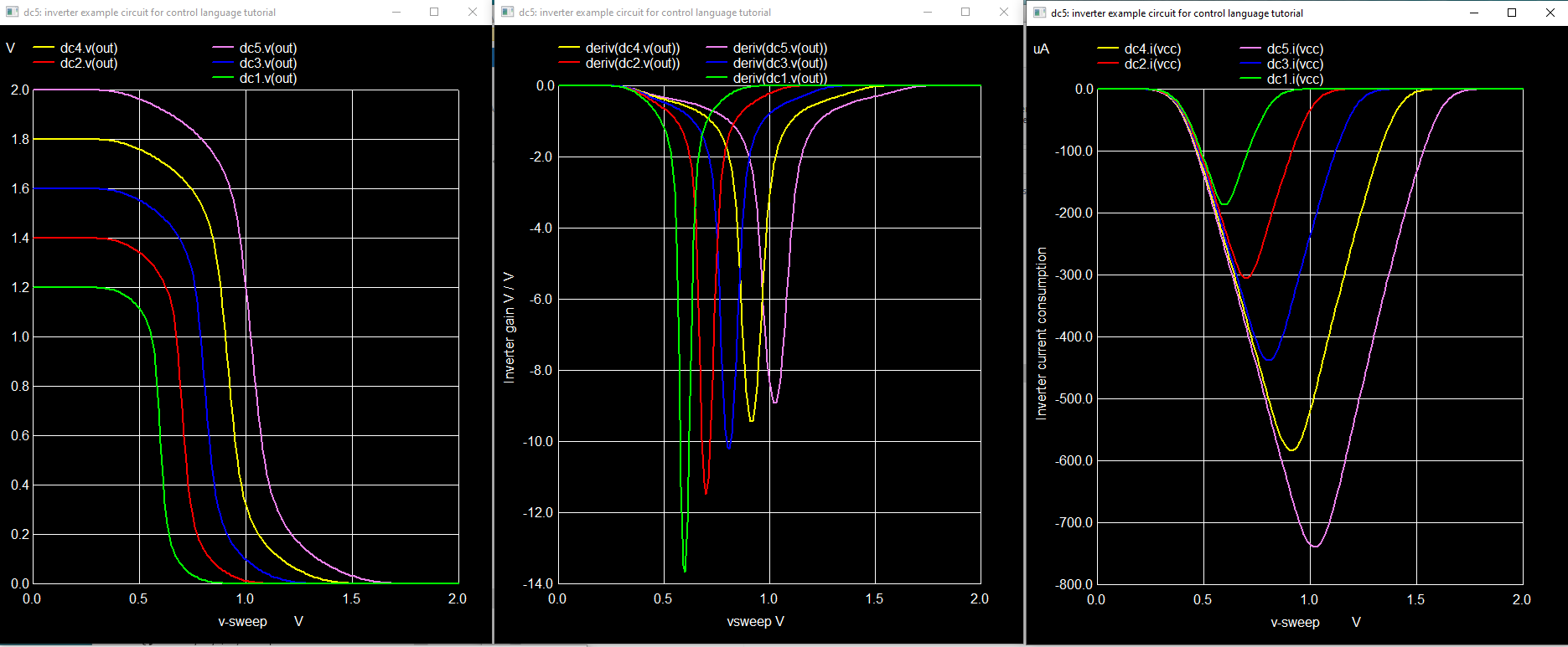
Fig. 2 Inverter output, gain and current consumption versus input voltage
Several new concepts are introduced in this script. Please refer to chapter 13.5
of the manual for details of the commands. repeat 5 ... end
will loop the enclosed commands five times. let vccc = 1.2 creates a vector (of length 1)
and assigns a value 1.2 to it. let vccc = vccc + 0.2 adds 0.2 to the current vector value.
alter Vcc $&vccc changes the voltage Vcc according to the value of vector vccc. $&vccc
returns the value of vector vccc. nounits and xbrushwidth are predefined variables (see manual chapter 13.7).
Command plot generates a graphical output by plotting one or several vectors versus a scale
vector (predefined is scale vector time for transient, v-sweep for dc). The results of
the last and all previous dc simulations are accessed by dc1.v(out) dc2.v(out) ....
This will be explained in the next paragraph. plot deriv(dc1.v(out)) uses function deriv,
returning the derivative of v(out) versus v-sweep (see manual, chapt. 17.2), therefore plotting the
voltage gain of the inverter. The supply current during dc sweep is measured as current out of the
voltage source Vcc, thus appearing negative.
4. About plots, variables and vectors
The output data of any simulation is available as vectors. An operating point simulation will create vectors of length 1, dc simulation will create vectors with length determined by the number of points during sweeping. These vectors are stored in plots, a traditional SPICE notion (see also chapter 13.3 of the manual). 'Plot' here is not to be confused with a plot resulting from plotting data. So a plot is a group of vectors. In our example the first dc command will generate several vectors within a plot dc1. A subsequent dc command will store their vectors in plot dc2 and so on. Transient simulation vectors would have been stored in plots tran1, tran2, etc. So each simulation command (dc, op, tran, sp ...) creates a new plot. The lastly created plot will stay active, until another plot is created or selected. There are also some functions creating their own plots, e.g. fft or linearize. The command setplot will show all plots and mark the active plot. For our example we have this
List of plots available:

Current dc5	inverter example circuit for control language tutorial (DC transfer characteristic)
	dc4	inverter example circuit for control language tutorial (DC transfer characteristic)
	dc3	inverter example circuit for control language tutorial (DC transfer characteristic)
	dc2	inverter example circuit for control language tutorial (DC transfer characteristic)
	dc1	inverter example circuit for control language tutorial (DC transfer characteristic)
	const	Constant values (constants)
with dc5 being the current plot. There is a pre-defined plot named const. It contains several constants.
Command display will name all vectors in the current plot. setplot dc2 will
switch the current plot to dc2.
Here are the vectors currently active:

Title: inverter example circuit for control language tutorial
Name: dc5 (DC transfer characteristic)
Date: Tue Jun  7 17:25:58  2022

    cc                  : voltage, real, 201 long
    in                  : voltage, real, 201 long
    out                 : voltage, real, 201 long
    v-sweep             : voltage, real, 201 long [default scale]
    vcc#branch          : current, real, 201 long
    vin#branch          : current, real, 201 long
[default scale] denotes the scale vector, which is used as x axis (during plotting or for calculating the derivative).
Vectors contain numbers (format double as real or complex numbers). They may contain a single value, be
one-dimensional or multi-dimensional. In the above example we have vectors of real numbers of length 201 each.
Vectors are local to their plot. You may access vectors from a different plot by prepending the plot name to
the vector name, separated by a dot, e.g. dc1.v(out) or dc2.I(vcc). Btw. I(vcc) is equal to vcc#branch, the branch
current through voltage source Vcc. The user may create their own vectors with the let command, e.g.
by let vccc = 1.2. As this command has been given before any simulation is run, the vector vccc will
reside in plot const. All vectors in plot const are globally available, no need to prepend anything.
Another class of storage elements is created by the ngspice variables. These are globally accessible
and may contain numbers, strings, or lists. There are pre-defined variables (see manual chapter 13.7) which
control many ngspice features. The command set will instantiate a variable and/or assign a content of it. in
our example we have used the pre-defined set xbrushwidth=2 to increase the plotting line width.
5. Looping a simulation, plot the maximum gain versus supply voltage
In the following example the loop is used to simulate and extract the inverter's voltage gain as function of its supply voltage. We simulate the output versus input of the inverter as a series of dc sweeps, the maximum gain for each voltage is determined and saved for plotting.
* control language script
.control
let loops = 6                     ; number of loops, vector in plot 'const'
let vecmaxgain = vector(loops)    ; vector in plot 'const'
let vecvcc = vector(loops)        ; vector in plot 'const'
let vccc = 1.0                    ; supply voltage in plot 'const'
let index = 0                     ; loop index in plot 'const'
repeat $&loops                    ; loop start
  alter Vcc $&vccc                ; alter the voltage Vcc
  dc vin 0 2 0.01                 ; run the dc simulation
  let gain = deriv(v(out))        ; calculate the gain
  let maxgain = vecmin(gain)      ; find the maximum of the gain (min because gain is negative)
  let vecmaxgain[index] = maxgain ; store the maximum gain
  let vecvcc[index] = vccc        ; store the corresponding voltage
  let vccc = vccc + 0.2           ; calculate new voltage value for Vcc
  let index = index + 1           ; raise the index
end                               ; loop end
destroy all                       ; delete all plot dc1 ..., no longer needed
set xbrushwidth=2                 ; linewidth of graph
set nolegend                      ; no legend on graph
plot vecmaxgain vs vecvcc xlabel 'Inverter supply voltage /V' ylabel 'Inverter gain V/V'
.endc                             ; end of control section
The vectors loops, vecmaxgain, vecvcc, vccc, and index are created in plot const, which is the current plot in the beginning of the script execution, before any simulation command is run. So these vectors will be accessible from within all plots created later by the simulation runs.
vector loops sets the number of loops and the size of the data storage vectors vecmaxgain
and vecvcc. repeat $&loops requires $&loops for reading the vector value.
During each simulation run the voltage Vcc is set, the dc simulation executed, the derivative of the output vector v(out) calculated, its maximum (minimum of the negative gain as function of the sweep voltage) determined and saved to the indexed location of vecmaxgain, together with vccc saved to vecvcc. Finally supply voltage and index are increased appropriately.
After the loop has ended, the command
destroy all deletes all plots created during dc simulation (dc1 to dc6).
They are no longer needed, so we save their memory. set nolegend supresses the legend,
because we have only a single vector plotted. plot vecmaxgain vs vecvcc plots
our new output (the max gain) versus the user selected scale, the corresponding supply
voltage.
An alternative to the destroy all is to delete only the most recent
(current) plot by destroy $curplot, now from inside the loop. curplot is another predefined variable
containing a string with the name of the current plot. Accessing the string is possible by
the prepended $.
...
  let index = index + 1           ; raise the index
  destroy $curplot                ; remove the current plot (created by dc...)
end                               ; loop end
set xbrushwidth=2                 ; linewidth of graph
...
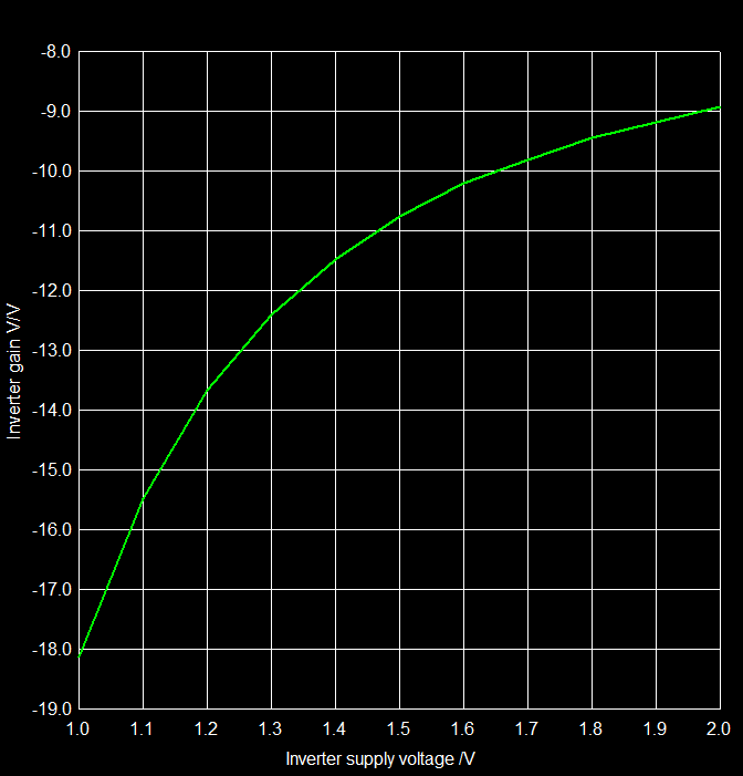
Fig. 3 is the final result. For smoothing the curve by more data points, the following commands have
been modified: let loops = 11 and let vccc = vccc + 0.1.
6. Looping the simulation as in 5., no plot, write data to file only
The inverter's voltage gain is determined as in the example above. The result is, however, not plotted, but written into a file as a simple table.
* control language script
.control
let loops = 11                    ; number of loops, vector in plot 'const'
let vccc = 1.0                    ; supply voltage in plot 'const'
repeat $&loops                    ; loop start
  alter Vcc $&vccc                ; alter the voltage Vcc
  dc vin 0 2 0.01                 ; run the dc simulation
  let gain = deriv(v(out))        ; calculate the gain
  let maxgain = vecmin(gain)      ; find the maximum of the gain (min because gain is negative)
  setscale vccc                   ; define the x axis (scale) with vector of length 1
  wrdata mgain.out maxgain        ; write out maxgain versus vccc for the current plot
  let vccc = vccc + 0.1           ; calculate new voltage value for Vcc
  destroy $curplot                ; remove the current plot (created by dc...)
  set appendwrite                 ; wrdata now adds data to existing file mgain.out
end                               ; loop end
.endc                             ; end of control section
wrdata writes vector(s) to a file as a simple table. Each vector is
written as a pair, first the scale (x axis value), then the output value. In our case the
output is maxgain (vector of length 1). The scale after a dc simulation is the voltage sweep.
This is not what we need here, as the scale for maxgain is vccc. So we use setscale vccc
to re-define the scale (before writing to file). wrdata creates a file or overwrites an existing
file with the current data. Here we use a trick: When entering the loop for the first time,
wrdata mgain.out maxgain creates the file mgain.out. Then, after first writing,
set appendwrite is issued. From then on, wrdata appends all data to the already
existing file. Calling set appendwrite several times does not hurt.
7. About loops in general
Several control structures are available for creating loops. Each loop starts with a keyword and ends with end. Nesting is supported. We use vectors (instatiated by let, de-referenced by $&, like $&loopindex) and variables (instantiated by set, de-referenced by $, like $val).
Here we have foreach...end and if...else...end:
foreach val -40 -20 0 20 40
  if $val < 0
    echo variable $val is less than 0
  else
    echo variable $val is greater than or equal to 0
  end
end
dowhile allows looping until a condition is fulfilled. The condition is tested after the statements
in the loop have been executed:
let loopindex = 0
dowhile loopindex <> 5
  echo index is $&loopindex
  let loopindex = loopindex + 1
end
We have already used the repeat loop:
set loops = 7
repeat $loops
  echo How many loops? $loops
end
while allows looping until a condition is fulfilled. The condition is tested befor the statements
are executed:
let loopindex = 0
while loopindex < 5
  echo index is $&loopindex
  let loopindex = loopindex + 1
end
In the
Sourceforge git examples for loops page you will find examples netlists for all loops,
ready to run. You may also have a look at the manual, chapter 13.6 on Control Structures,
where additionally the commands label, goto, break and
continue are described.
8. String substitution
Vectors contain numbers. They may be one-dimensional (often with only a single element, aka length = 1) or multi-dimensional. Variables may contain integer or real numbers, strings, a boolean yes, or a list of elements as strings.
Both are used in the following script as part of new variables. Substitution is done by replacing the {} with the contents of the vector or variable element named inside of the {}.
*ng_script                ; this is a script only
.control
* simple replacement
let ii = 1                ; new 1D vector containing value 1
set myplot = tran2        ; new variable containing a string
* substitution
set subs1 = {$myplot}.out ; {} is substituted by string of variable myplot
set subs2 = dc{$&ii}.in   ; {} is substituted by vector contents converted to string
echo $subs1 $subs2        ; print both variables

* somewhat more complex substitutions
let vec = vector(6)             ; new vector with 6 elements, numbered from 0 to 5
set myplots = ( tran3 dc5 op1 ) ; new variable with list of 3 elements, numbered from 1 to 3
let vec4 = vec[4]               ; intermediate stage, read vector element 4 into a new vector.
set subs3 = {$myplots[3]}.out   ; {} is substituted by element 3 of string list in variable myplots
set subs4 = dc{$&vec4}.in       ; {} is substituted by vector contents converted to string
echo $subs3 $subs4              ; print both variables

.endc
.end
The outputs echoed to the console are:
tran2.out dc1.in
op1.out dc4.in
Some comments to this script are due: *ng_script in the upper left of the first row will tell ngspie
that a pure script is following, thus skipping any circuit parsing. Substitution may happen with a
single element from a vector or variable. Elements of a vector are numbered by 0 to number-of-elements - 1,
elements of a string list in a variable are numbered 1 to number-of-elements. Elements of a vector may be used
for substituting only after an intermediate step of converting them to a vector of length 1. When
defining a list variable, take care for spaces between ( or ) and the elements.
9. Nested loops
In the following netlist there is a very simple circuit: 3 resistors in series, powered by a voltage source. We want to change each resistor using the alter command. We use 3 interlaced while loops.
3 interlaced while loops, simple circuit

R1 1 11 1
R2 11 12 1
R3 12 0 1

V1 1 0 1

.control
* initialization (vectors in plot const)
let rsta1 = 1k
let rsto1 = 5k
let rste1 = 1k
let rsta2 = 200  ; start value for R2
let rsto2 = 1000 ; stop value
let rste2 = 200  ; step value
let rsta3 = 20
let rsto3 = 200
let rste3 = 20
let rloop1 = rsta1
let rloop2 = rsta2 ; loop value for R2
let rloop3 = rsta3
* three nested while loops
while rloop1 < rsto1
  alter R1 rloop1
  while rloop2 < rsto2
    alter R2 rloop2 ; modify R2 by current rloop2 value
    while rloop3 <= rsto3
      alter R3 rloop3
      op
      let rtotal = rloop1 + rloop2 + rloop3
      echo $&rloop1 $&rloop2 $&rloop3 $&rtotal $&V1#branch
      let rloop3 = rloop3 + rste3
    end
    let rloop3 = rsta3
    let rloop2 = rloop2 + rste2 ; calculate new rloop2 value
  end
  let rloop2 = rsta2            ; reset rloop2 to its start value
  let rloop1 = rloop1 + rste1
end
rusage
.endc

.end
For varying each resistor, each resistor gets its vectors for the start, stop and step values.
The three rloop vectors will be varied during looping. One has to be careful where to place the
command lines alter R2 rloop2, and let rloop2 = rloop2 + rste2. Right
after a loop has finished, its corresponding rloop vector has to be reset to its start value,
e.g. by let rloop2 = rsta2 again.
10. Emulate nested .step commands
Creating nested loops and running several simulations in series without external intervention are a powerful tool to characterize circuits. Currently unfortunately ngspice does not offer the .step command, which may simplify setting up such simulation loops. However the control language allows to emulate such behaviour. The netlist below will emulate code like
.step lin R1 list 10k 20k 30k
.step lin C2 list 1u 0.5u 0.25u
.step lin R2 list 1m 3.3k 6.6k
In the future ngspice may be enabled to translating such .step commands into
emulating control sections automatically
and transparent to the user, so simplifying their job. For now we may use such a netlist for
learning about some new features of the control language.
* .step emulation: 3 nested loops, ac simulation
* R1, C2 change by param, R2 changes directly
* loops by foreach
* commands alterparam, alter: all three alter commands inside of inner loop
* alterparam first, followed by reset, only then followed by alter
* print out the results into a file threeloopsac.txt, located in the input
* directory (where this netlist has been found).

.param rr1 = 1k cc2 = 1u

V1 1 0 dc 0 ac 1
R1 1 11 {rr1}
R2 11 10 100
C2 10 0 {cc2}

.ac dec 10 1 1e4

.control
let index = 0        ; new loop index vector (in plot 'const')
set plotstrdb = ' '  ; new variable containing string with space (will become a list of strings, see below)
set plotstrph = ' '  ; new variable containing string with space (will become a list of strings, see below)
set writestr = ' '   ; new variable containing string with space (will become a list of strings, see below)
set cvalues = ( 1u 0.5u 0.25u ) ; variable containing loop values for C2

** loop start **
foreach val1 10k 20k 30k                                    ; outermost loop with a value list
  foreach val2 $cvalues                                     ; loop in the middle with a variable containing a value list
    foreach val3 1m 3.3k 6.6k                               ; inner loop with a value list
      let index = index + 1                                 ; raise loop index
      echo ac sim no. $&index',' R1=$val1',' R2=$val3',' C2=$val2 ; print to console where we are
      alterparam rr1 = $val1                                ; change parameter of outer loop
      alterparam cc2 = $val2                                ; change paramater of middle loop
      reset                                                 ; reset to activate above parameter changes
      alter R2 $val3                                        ; change inner loop value (possible only after reset!)
      run                                                   ; run the simulation (see .ac ... above)
      set plotstrdb = ( $plotstrdb db({$curplot}.v(10)) )   ; add a new item (string) to already exising list of strings
      set plotstrph = ( $plotstrph cph({$curplot}.v(10)) )  ; add a new item (string) to already exising list of strings
      set writestr = ( $writestr {$curplot}.v(10) )         ; add a new item (string) to already exising list of strings
    end
  end
end
** loop end, start plotting **
set nolegend                  ; legend for 27 graphs is unreadable
set units=degrees             ; phase in degrees
set xbrushwidth=2             ; increase linewidth of graphs
plot $plotstrdb xlimit 1 1e4  ; plot all 27 magnitudes
plot $plotstrph xlimit 1 1e4  ; plot all 27 phases
set wr_singlescale            ; for wrdata: write the scale only once
set wr_vecnames               ; for wrdata: write the vector names
option numdgt = 3             ; for wrdata: 3 digits after decimal point
wrdata $inputdir/threeloopsac.txt $writestr  ; write ac output v(10) into file for all runs
rusage                        ; list some resource usage
.endc

.end
Fig. 4 is what you get with the two plot commands:
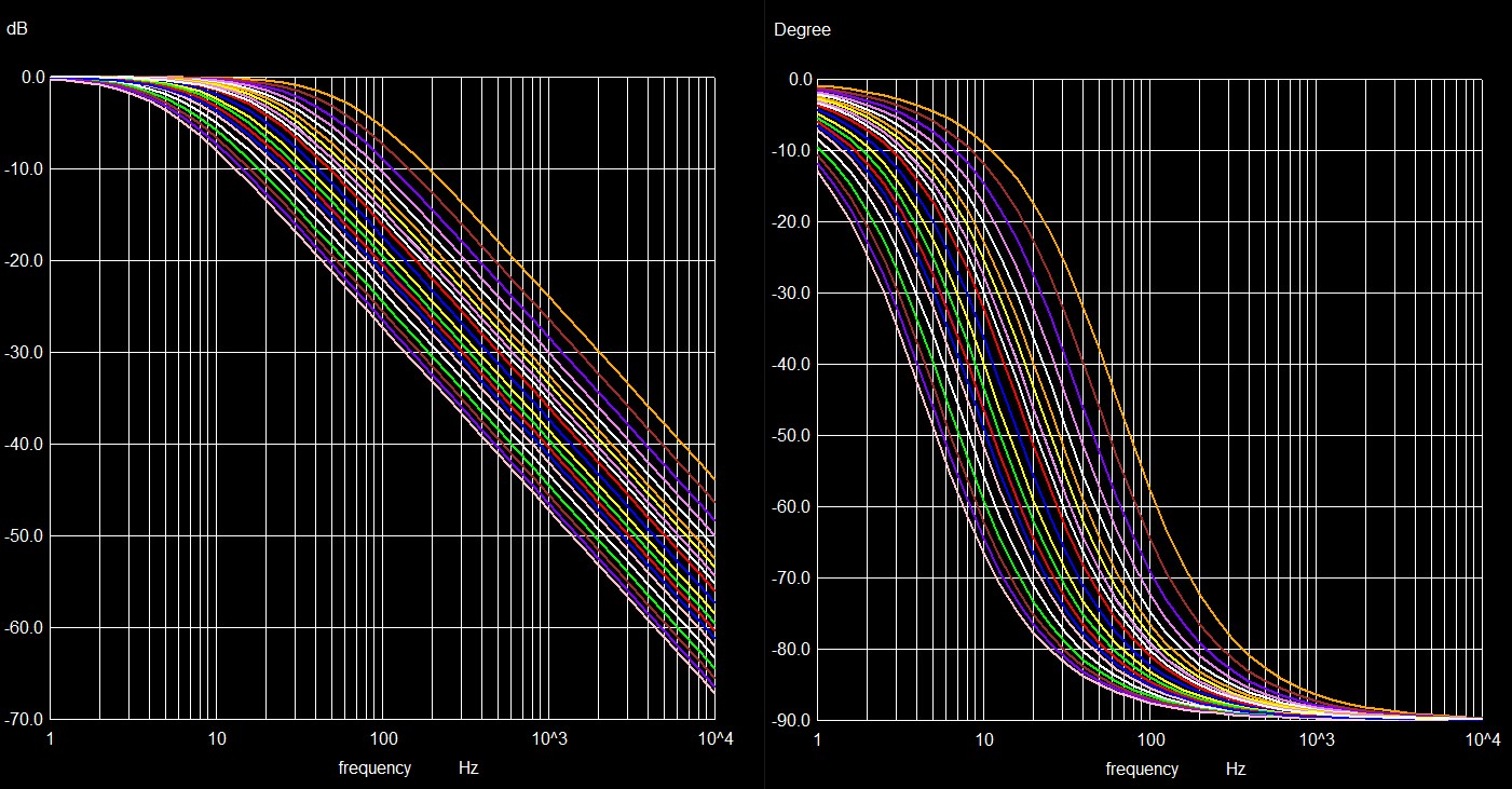
Fig. 4 Gain and phase of RC circuit, 27 simulation runs in total
The output file, written by command wrdata, looks like this:
 frequency  ac1.v(10)  ac1.v(10)  ac2.v(10)  ac2.v(10)  ac3.v(10)  ac3.v(10) ...
 1.000e+00  9.961e-01 -6.258e-02  9.931e-01 -8.299e-02  9.892e-01 -1.032e-01 ...
 1.259e+00  9.938e-01 -7.861e-02  9.891e-01 -1.041e-01  9.831e-01 -1.291e-01 ...
 1.585e+00  9.902e-01 -9.860e-02  9.828e-01 -1.302e-01  9.734e-01 -1.609e-01 ...
 1.995e+00  9.845e-01 -1.234e-01  9.730e-01 -1.622e-01  9.585e-01 -1.995e-01 ...
...
The first column is the frequency, the next 2 columns are the real and the imaginary parts of complex vector v(10) from plot ac1, then follow real and imaginary parts of vector V(10) from plot ac2 etc.
Some comments also here: The circuit is simply two resistors in series (R1 + R") with capacitor C2 from output v(1) to ground, a low pass filter. We set three variables in the beginning, each containing just a space. '...' delimit a string, even if it contains specal characters (e.g. a space). Three nested foreach loops are used with a value list or with a variable containing such a list. The echo command in the loop again uses '...' for formatting. Otherwise spaces or commas would just be swallowed and replaced by a single space. The alterparam command has to be followed by a reset command to become activated. On the other hand alter commands are resetted by reset. Therefore all three altering commands have to be in the inner loop, repeated each time the loop is executed. Any alterparam has to come first, then reset, only then any alter (or altermod) commands.
set plotstrdb = ( $plotstrdb db({$curplot}.v(10)) ) requires some
explanation: {$curplot}.v(10) substitutes the {} with the name of the current plot (e.g. ac3),
just to obtain ac3.v(10). This string, embedded in db(...) is added to the variable plotstrdb,
increasing its string list. In the beginning plotstrdb started with a space, then one item is added per loop,
e.g. yielding db(ac1.v(10)) db(ac2.v(10)) db(ac3.v(10)) ....
Another group of .step commands loops the temperature and device parameters given by
a start, stop and step value for each parameter, like
Again there are three nested loops, but now we use the while ... end loop command.
* .step temp -55 125 10
* .step npn 2N2222 (VAF) 50 300 50
* .step param R1 2k 10k 2k
*** Emulate the .step command

.param ptemp = -55 R1 = 2k
.temp {ptemp}                      ; set the overall circuit temperature

V1 vcc 0 5                         ; the circuit
R1 vcc cc {R1}
Q1 cc bb 0 BC546B
R2 vcc bb 500k

.probe I(Q1)                       ; measure the Q1 terminal currents
.save all                          ; not only save the Q1 current values, but all node values

.op

.control
let index = 1                       ; new loop index vector (in plot 'const')
let tcur = 25                       ; new temperature vector (in plot 'const')
while tcur <= 125                   ; the temperature loop
  let mvaf = 50                     ; new model parameter vector (in plot 'const')
  while mvaf <= 300                 ; the VAF loop
    let rr1 = 2k                    ; new resistance parameter vector (in plot 'const')
    while rr1 <= 10k                ; the resistor R1 loop
      echo
      echo
      echo *** op no. $&index',' R1=$&rr1',' VAF=$&mvaf',' temp=$&tcur *** ; print to console where we are
      alterparam ptemp = $&tcur     ; change the temperature parameter
      alterparam R1 = $&rr1         ; change the R1 resistance parameter
      reset                         ; activate the parameter changes by reloading the ciruit
      altermod BC546B VAF = $&mvaf  ; change the VAF model parameter
      run                           ; run the op simulation
      print v(cc) v(bb) i(q1:c) i(q1:b) ; the data output, i(q1:c) is the same as q1:c#branch
      let rr1 = rr1 + 2k            ; new resistance value
      let index = index + 1
    end
    let mvaf = mvaf + 50            ; new VAF value
  end
  let tcur = tcur + 10              ; new temperature value
end
display
rusage
.endc

*From Philips SC04 "Small signal transistors 1991"
* Base spreading parameters (RB,IRB,RBM) estimated. TR derived using BCY58 data
.model BC546B npn ( IS=7.59E-15 VAF=73.4 BF=480 IKF=0.0962 NE=1.2665
+ ISE=3.278E-15 IKR=0.03 ISC=2.00E-13 NC=1.2 NR=1 BR=5 RC=0.25 CJC=6.33E-12
+ FC=0.5 MJC=0.33 VJC=0.65 CJE=1.25E-11 MJE=0.55 VJE=0.65 TF=4.26E-10
+ ITF=0.6 VTF=3 XTF=20 RB=100 IRB=0.0001 RBM=10 RE=0.5 TR=1.50E-07)

.end
So what is new here? Command .temp {ptemp} sets the overall circuit temperature
to the value of parameter ptemp. We now use an active device, the npn bipolar transistor Q1, whose model
parameters are given in the .model BC546B npn ... line. The .probe(Q1) command allows to measure
the device Q1 terminal currents as shown by the display command:
The three nested loops start with while tcur <= 125. One has to be careful where to place correctly
the initial loop value let tcur = 25 and the command let tcur = tcur + 10 to increase the value.
Changing the model parameter VAF (forward Early voltage) is done by altermod, again after setting
the parameters by alterparam and after reset. Data output is provided here by the simple
print command.
    q1:b#branch         : current, real, 1 long
    q1:c#branch         : current, real, 1 long
    q1:e#branch         : current, real, 1 long
The above netlist implicitely provides a linear increase of parameters. A .step command like
with its option oct implies a non-linear distribution of input parameters (here 5 values per octave,
that is within a factor of 2). A netlist with a single loop demonstrates this command:
* .step oct v1 1 100 5
Here we use a multiplicator to alter the voltage value, derived from the information "5 values
per octave". After calculating the total number of steps, we create and use 2 vectors vecx, vecy
to store the result of the op simulation versus the V1 value. Some checking against
wrong point numbers is done. A pointplot in Fig. 5 demonstrates the uniform x value distribution,
when plotted logarithmically.
*** Emulate the .step command
* .step oct v1 1 100 5

V1 vcc 0 1                          ; the circuit
R1 vcc 0 1

.op                                 ; simulation type required

.control
let vstart = 1                      ; start voltage vector (in plot 'const')
let vend = 100                      ; end voltage vector (in plot 'const')
let numb = 5                        ; number of points per octave (in plot 'const')

let index = 1                       ; new loop index vector (in plot 'const')
let vmult = 2^(1/numb)              ; multiplicator

let xx = vend/vstart                ; find the total number of steps
let ind1 = 0
while xx > 1
  let xx = xx / vmult
  let ind1 = ind1 + 1
end
echo number of steps $&ind1

if ind1 < 1                          ; move on when number of steps is positive
  echo error with number of steps $&ind1 --'>'  stop!
else
  let vecx = vector(ind1)            ; create vectors for x and y
  let vecy = vector(ind1)
  settype voltage vecx               ; set the correct vector type
  settype current vecy

  let vcur = vstart                   ; current voltage value in the loop
  while vcur <= vend                  ; the voltage loop
    alter V1 vcur                     ; a new voltage value for V1
    echo run no. $&index
    run                               ; simulate
    let indloc = index - 1            ; indexes for vectors start with 0
    let vecx[indloc] = vcur           ; x value into vector
    let vecy[indloc] = v1#branch      ; y value into vector
*    print vcur v1#branch
    unlet indloc                      ; remove vector no longer used
    echo
    let vcur = vcur * vmult           ; calculate new voltage value
    let index = index + 1
  end
  plot vecy vs vecx pointplot xlog    ; plot y versus x
end
rusage                                ; memory and time used
.endc

.end
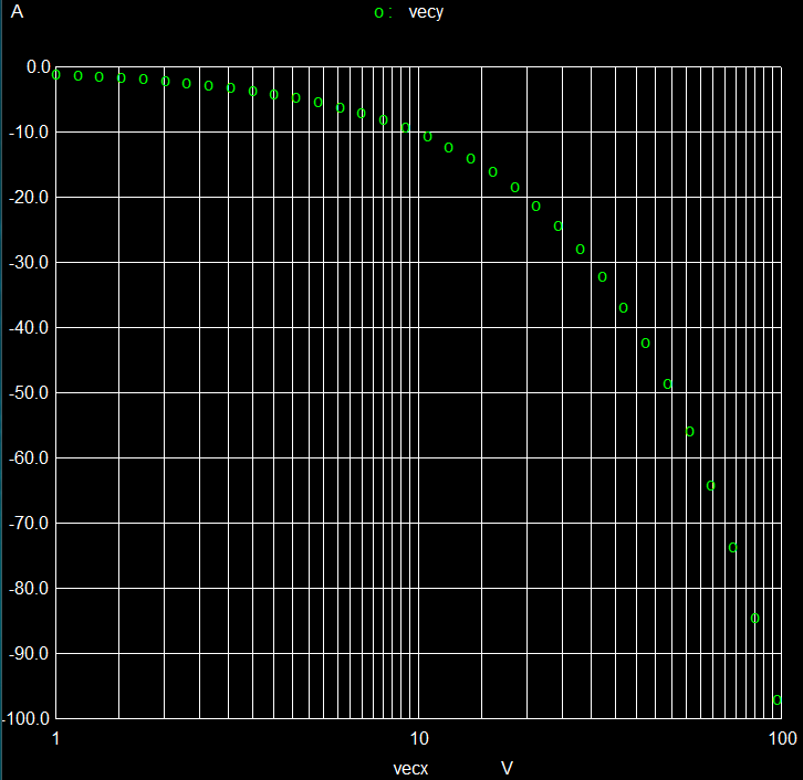
Fig. 5 Output current versus logarithmic voltage value distribution
11. Modify a circuit on the fly
By using the .if ... .elseif ... .endif construct, you may choose from
different circuit blocks which are enclosed within the conditional statements. Selection
is done by altering a parameter as selector with the alterparam command.
In the first example we switch between a simple low pass and a high pass circuit, run an .ac simulation for each one and plot the output in a single plot window.
High pass, low pass on the fly

.param select = 0          ; selector

.IF (select == 0)          ; select low pass
    R1 in out 1k
    C1 out 0 1u
.ELSEIF (select == 1)      ; select high pass
    R1 out 0 1k
    C1 in out 1u
.ENDIF

Vin in 0 dc 0 ac 1         ; input voltage

.ac dec 10 1 100k

.control
run                        ; run the simulation
alterparam select = 1      ; modify the selector from 0 to 1
reset                      ; reload the circuit with new selector, so with new circuit
run                        ; run the simulation again
set xbrushwidth=3          ; increase linewidth of graphs
plot db(ac1.out) db(ac2.out) xlimit 1 1e5 ; plot both simulations in one graph
.endc

.end
Some restrictions apply, as the following netlist components are not
supported within the .IF ... .ENDIF block: .SUBCKT, .INC, .LIB, and .PARAM.
In the next example we choose from 2 different operational amplifiers. We have to include all of their models, and we select by calling the appropriate model in the call to their subcircuit (X line).
* Modify circuit (here: changing OpAmps) using .IF ... .ENDIF

.param select = 0                ; selector

.IF (select == 0)                ; select OpAmp
    X1 0 INM P6V M6V OUT OPA1656
.ELSEIF (select == 1)
    X2 0 INM P6V M6V OUT OPA164x
.ENDIF

R1 INM OUT 10K                    ; inverting amplifier, gain -2
R2 IN INM 5k

V1 P6V 0 4V                       ; power supply
V2 M6V 0 -4V

Vin IN 0 dc 0 ac 1                ; input (for ac)

.ac dec 20 1e4 1e8                ; ac simulation conditions

.include OPA1656.lib ; download OpAmp model from TI's web site
.include OPA164x.lib ; download OpAmp model from TI's web site

.control
save out                   ; save only the output, all other nodes are discarded
run                        ; run the simulation
alterparam select = 1      ; modify the selector from 0 to 1
reset                      ; reload the circuit with new selector, so with new OpAmp
run                        ; run the simulation again

let dbout1 = db(ac1.out)   ; calculate db in preparation for meas command, previous run
let dbout2 = db(out)       ; calculate db in preparation for meas command, current run
set xbrushwidth=3          ; increase linewidth of graphs
plot dbout1 dbout2
meas ac fmin3db1 when dbout1=3 ; gain 6 dB, measure fall-off to 3 dB
meas ac fmin3db2 when dbout2=3 ; gain 6 dB, measure fall-off to 3 dB
.endc

.end
Finally we use two meas(ure) commands to find the frequency where
the opamp gain has rolled off by -3 dB.
The results of both simulations are presented in Fig. 6:
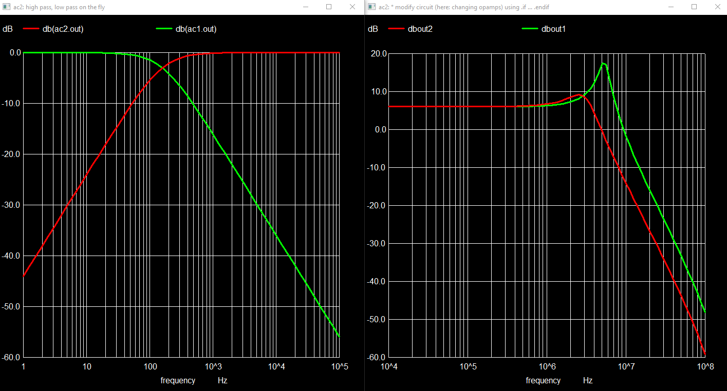
Fig. 6 Gain of RC circuit and two operational amplifiers versus frequency
12. More examples
A lot of example netlist are provided with the ngspice distribution. You may also find them in our Sourceforge git pages. Especially the Monte Carlo simulations make heavy use of more or less complex control scripts. As an external source, provided by astx, scripts are published for completely characterizing audio amplifiers. See the thread installing-and-using-ngspice at diyAudio.
